The structure of a Mathematica package

I like to build tools to make programming easier.

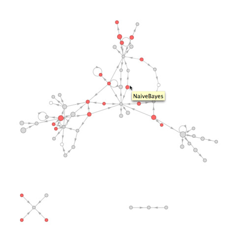
One of my latest tools is a useful function that plots the “call graph” of a Mathematica package: each vertex is a function, and each represents the fact that the one function calls another. It’s a neat way to understand the structure of a large body of a code without “chasing down” function calls by hand.

For example, the graph below¹ shows the structure of a machine learning package I’m writing. The size of the disks show function code size — bigger disks for more complex functions. Interestingly, Mathematica allows me to measure this directly, rather than using the usual proxy of the number of lines in the source code for a function. By taking the LeafCountreference.wolfram.com of the DownValuesreference.wolfram.com of a symbol, I get the number of independent parts in the abstract syntax tree of a function.

Other visual elements also communicate important details: red disks are public functions — functions that the package exports to external code. White disks, conversely, represent functions imported from other packages. And lastly, recursive functions (by definition) are those vertices with a circular edge that loops back to thesmelves.