Projects / Biologically plausible backprop

SOAP (Second Order Activity Perturbation) is a package for experimenting with a computational neuroscience phenomenon called feedback alignment in PyTorch. It formed my project for the 3-week IBRO-Simons Computational Neuroscience Summer Schoolimbizo.africa in 2019. It relates to an important challenge in reconciling how learning works in artificial neural networks with what we know about how real neurons behave, a topic called biologically plausible back-propogation.

Backprop and learning

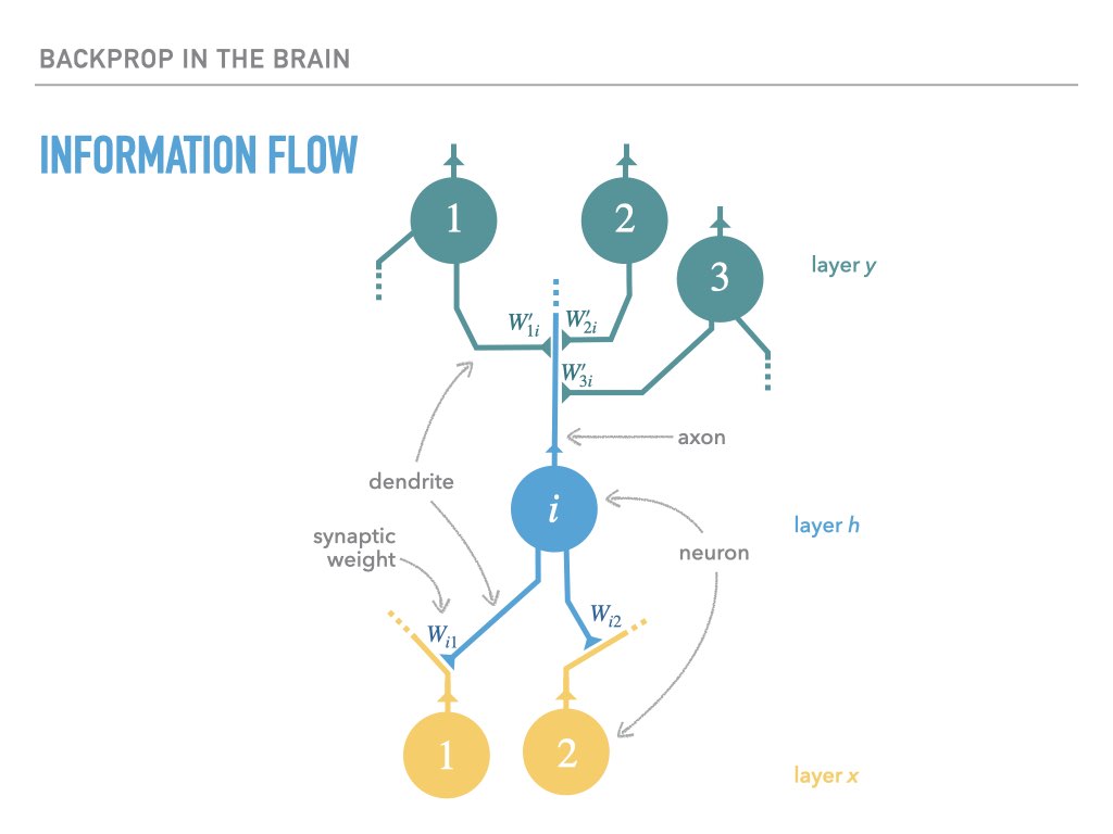
When a neuron fires, its axon transmits a voltage spike that is received by downstream neurons whose dendrites interface with the axon via a synaptic cleft. If the type of connection is excitatory, this spike makes the downstream neurons more likely to fire; if the connection is inhibatory, the downstream neurons become less likely. The strength (or even absense) of a connection between two neurons is often called a synaptic weight:

A learning process that is accomplished via some kind of error signal needs to somehow ensure that the synaptic weights of neurons change in such a way as to reduce the error signal over time.

Artificial neural networks that are trained by backpropogation can precisely define the infinitesemal influence of each synaptic weight on an downstream error signal (called loss) via the technique of reverse-mode automatic differentiation (this is back-propogation). This allows us to compute the gradient with respect to a training loss, allowing weights to change such as to lower this loss:

For a single layer of neurons, the exact calculation of gradients is accomplished as follows, where we use the notation $\dot x = \ifrac {\partial L}{\partial x}$, with $L$ being the loss:

The weight transport problem

The problem is that biological neural networks can’t work this way! The orange arrows that carry the gradient signal backwards through the network cannot be implemented by the same axons involved in the forward pass, since these are one-way communication channels. But if a different circuit carried these error signals back to pre-synaptic neurons, it would not have access to the synaptic strengths that went into making the given neuron fire, and so there is no way for the neuron to compute the correct vector-Jacobian product that is required to perform back-propogation through a layer to calculate the gradient required for previous layers. From the slides:

Feedback alignment

In 2016 Lillicrap et al noticed that instead of using the transpose of the weight matrix needed for $\dot W$, we can instead use a fixed random matrix $B$:

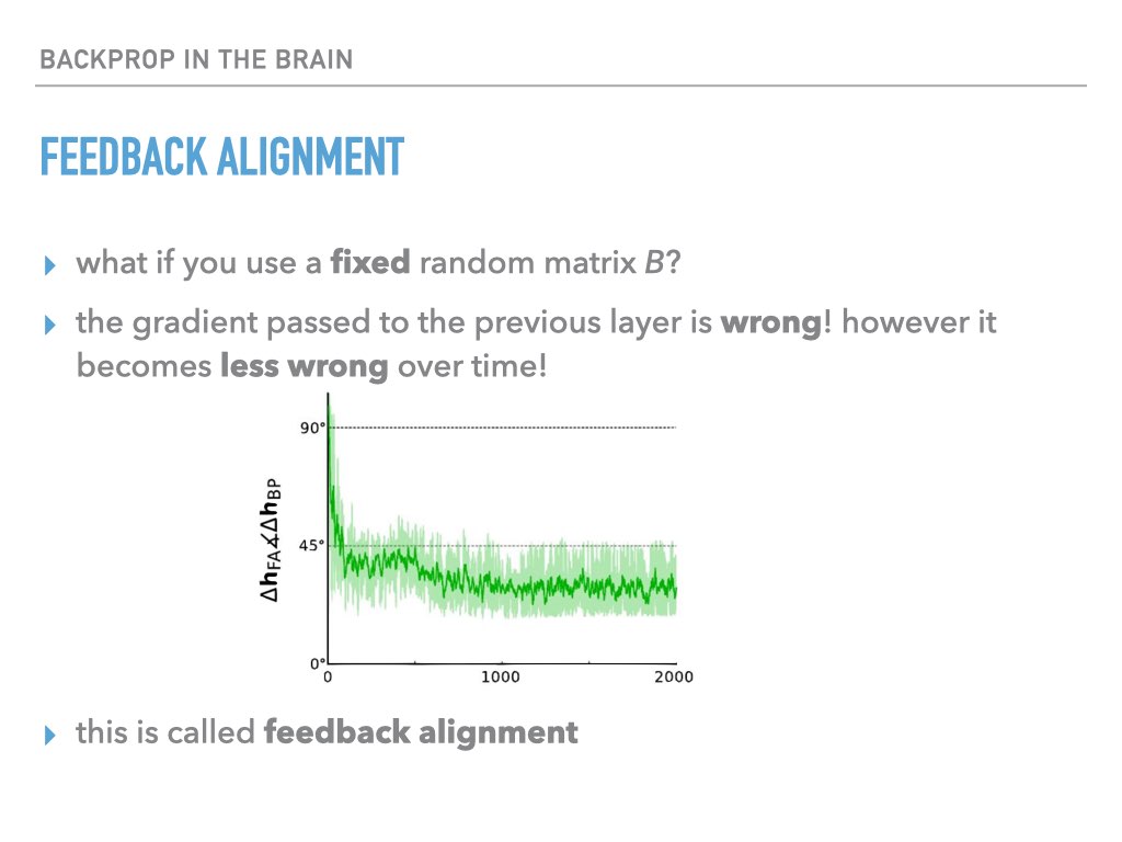
Surprisingly, this works, and it works better over time. Effectively, the weight matrix W learns how to compensate for B being incorrect. For more information on Feedback Alignment, see Lillicrap’s original paper¹, which contains arguments for what might be going on.

Vanilla feedback alignment

To start, I wanted to get feedback alignment training an MLP on MNIST. Using a modern framework like pytorch this turns out to be pretty easy to do, though slightly more verbose than I would expect. We can write a FeedbackAlignmentLinear layer that behaves like the standard Linearpytorch.org for the forward pass, but uses a custom, random B-matrix to backpropogate gradients:

class FALinearFunction(Function):

    @staticmethod
    def forward(ctx, data_in, weight, bias, b_matrix):
        ctx.save_for_backward(data_in, weight, bias, b_matrix)
        return data_in.mm(weight.t()) + bias.unsqueeze(0).expand_as(data_in)

    @staticmethod
    def backward(ctx, grad_out):
        data_in, weight, bias, b_matrix = ctx.saved_tensors
        return grad_out.mm(b_matrix), grad_out.t().mm(data_in), grad_out.sum(0), None

class FALinear(nn.Module):
    def __init__(self, num_in, num_out):
        super().__init__()
        self.weight = nn.Parameter(torch.Tensor(num_out, num_in))
        self.bias = nn.Parameter(torch.Tensor(num_out))
        b_matrix = torch.zeros(num_out, num_in)
        self.register_buffer('b_matrix', b_matrix)
        init.xavier_normal_(b_matrix)
        init.xavier_normal_(self.weight)
        init.uniform_(self.bias, 0, 0)

This layer does indeed train on MNIST, though more slowly than standard back-propogation:

Although the two curves above look close, drawing a horizontal line through both curves shows that FA takes roughly twice as long to reach a given loss as BP — at least on this particular run.

Can we improve on this?

Improving on FA

Muskovitz et al showed² that we can improve FA by “breaking the rules” a bit: instead of allowing no weight transport, we can allow a little bit of information to periodically leak into the B matrix.

Let’s start with one bit of information leaking into $B$ from $W$, per neuron: merely the sign of the transpose of the weight matrix, updated only every $T$ examples rather than after every example.

We can write this as $B_t \leftarrow \operatorname{sign}(W_t^T)$ where $t \in \{T, 2T, 3T, \ldots\}$.

We indeed get quite a jump in performance. This sign-sychronized feedback alignment appears to outperform backprop, which is quite surpising!

Unfortunately this single run is misleading. There is a subtle effect here, having nothing nothing to do with feedback alignment, which is actually responsible for this increased performance. It is related to learning rates: for this run we happened to have picked an SGD learning rate that was lower than optimal. Our update rule for $B$ has the effect of amplifying the (pseudo)gradient signal, an effect that more than compensates for the inaccuracy of using an incorrect gradient.

We can remove this effect by modifying the update rule to $B_t \leftarrow |B_0| \operatorname{sign}(W_t^T)$, so that the magnitude of the original feedback weights is preserved. Sure enough, the performance gain largely disappears, and this form of FA is still worse than ordinary back-propagation:

The following causal diagramWikipedia captures the confounding effect that the naive sign-change learning rule has on the model performance by modifying the average effective learning rate. In the language of casual diagrams, effecive learning rate is part of a collider; once we mask the influence of the learning rule on the effective learning rate, the influence of the learning rule on model accuracy mostly dissappears for this particular experiment, casting doubt on the conclusion. It would not be enough to simply adjust the imposed learning rate, since the magnitude of the learned weight matrix could adjust arbitrarily to compensate in the same way it adjusts to compensate for proxy matrix B being wrong.

This simple result, which undermined one of the inspirations for the project, cast doubt for me on the prospect of concluding anything meaningful from the actual experiments that I did do! Because we do not usually have a good understanding on how a given test problem could or should be solved by a learning algorithm, it is hard to conclude much about the reasons for improved performance when we try something new. But what in fact did I try?

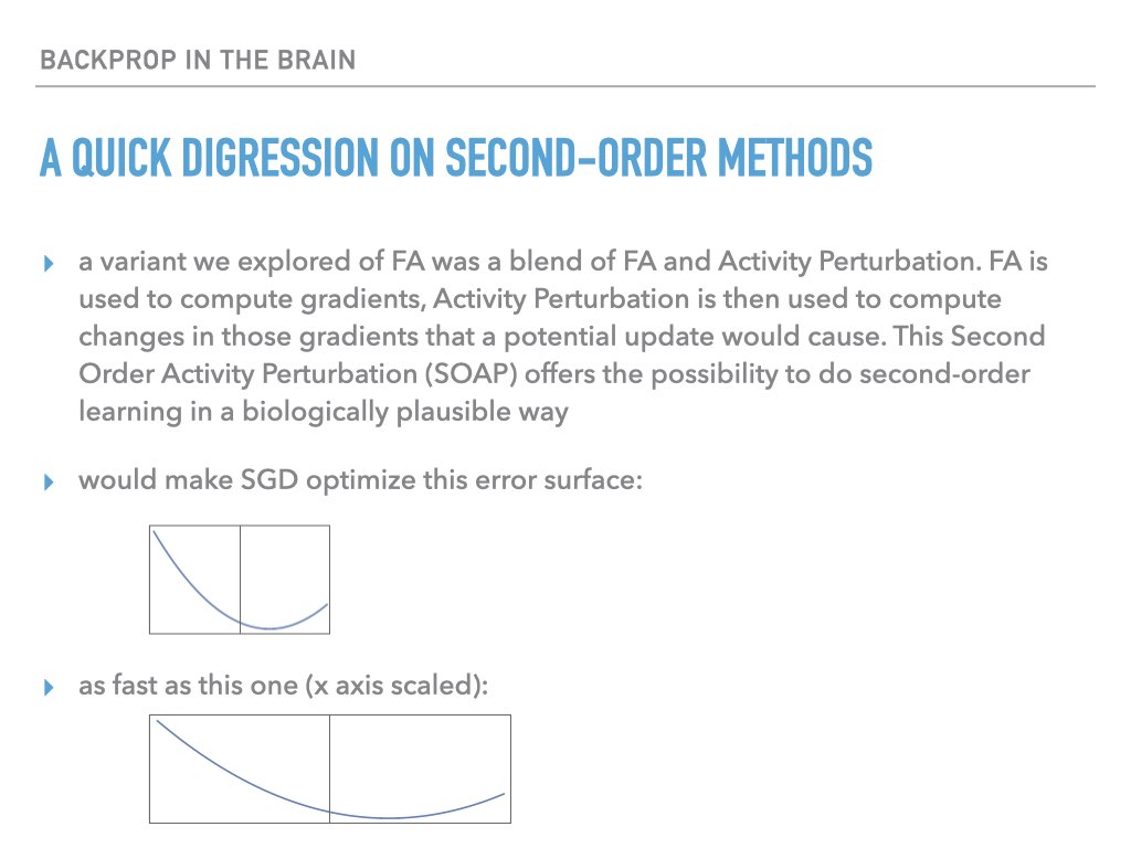
Exploiting curvature

The idea I originally intended was to combine feedback alignment with activity perturbation (also called node perturbation). Activity perturbation effectively computes the gradient using temporal dynamics, whereby several forward passes with intrinsic noise can be used to approximate the gradient. It doesn’t work very well because the chances that the noise will align with the direction in parameter space corresponding to the true gradient are vanishingly small. But my idea was that once we had a good estimate of the gradient from feedback alignment, we could use this same “temporal finite difference” method to achieve a much better gradient estimate that effectively exploited curvature of the loss landscape (eigenvectors of the Hessian matrix). This is analogous to Newton’s method for improving the convergence rate of iterative root-finding.

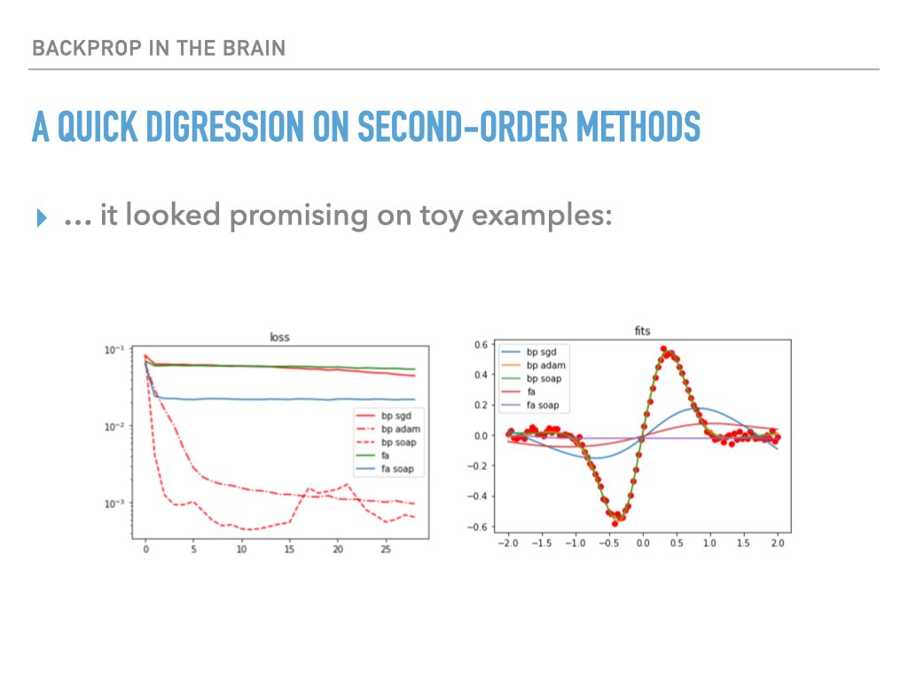
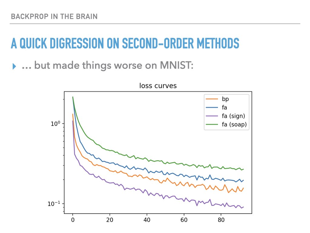
My findings were mixed on toy examples, and the experience with rescaled feedback alignment (see above) left me skeptical that even positive results could be used to conclude anything significant about whether second order information was being exploited:

Summary

In a way, this project was a failure, because even after writing some fun code and doing some experiments that seemed promising at first, the underlying evaluation methodology came under suspicion. I think this is a criticism that can be made of a lot of typical computational neuroscience and deep learning research, though certainly not all! It did leave me much less enthusiastic to “play around with architectures and algorithms” until we had a better understanding of the solution space itself that our algorithms are exploring.