SGT is a Mathematica package to unlock effortless explorations in evolutionary spatial game theory. Using SGT, you can setup, conduct and visualize experiments using a small number of functions and symbolic expressions to specify the initial distribution of agents, the topology of the grid, the strategies the agents employ, the payoff structure of the games they play, the rules used to update the agents and apply natural selection, whether and how mutation occurs, whether agents have access to more or less information about their opponents, and whether their success depends on global as well as local properties.

This work is primarily inspired by the work of Martin Nowak at the Program for Evolutionary Dynamicswww.ped.fas.harvard.edu.

Gallery

The following examples demonstrate how the spatial patterns of agents that are playing various types of games evolve over time. Most of these examples incorporate agents that merely play the same strategy again and again, this corresponds to the AgentType -> "Constant" option in the corresponding code. From each simulation, snapshots are shown of the spatial patterns at various times (indicated by the “t = …” legend).

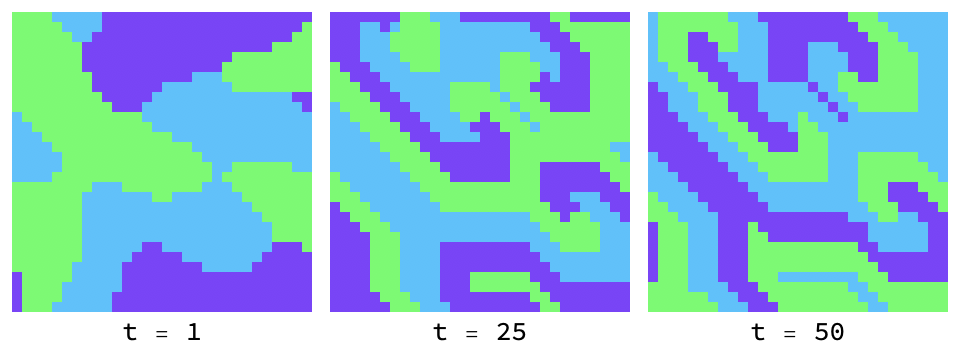
Rock paper scissors

Simulate[
	InitialPopulation -> Randomized[{-1, 0, 1}, "Smoothing" -> 1],
	Payoff -> RockPaperScissors, AgentType -> "Constant",
	Steps -> 1 ;; 100]

Domains of rock (light blue), paper (green) and scissors (dark blue) chase each other around endlessly, as there is no evolutionary stable strategy:

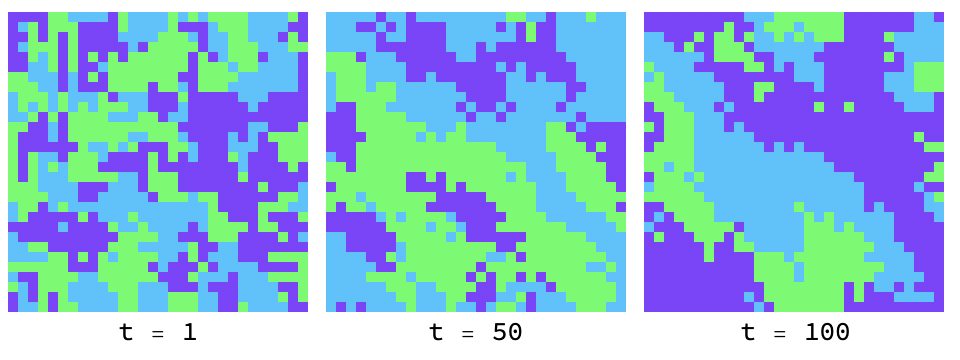
Low temperatue and smoothed initial conditions give rise to what looks very much like the BZ reactionen.wikipedia.org in chemistry:

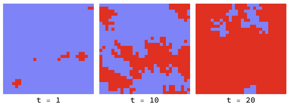
Prisoner’s dilemma

Simulate[
	InitialPopulation -> 
	Randomized[{1, 1} -> {-1, 1}, "Smoothing" -> 2],
	Payoff -> PrisonersDilemma, AgentType -> "Constant",
	Neighborhood -> 8, Temperature -> 1/5]

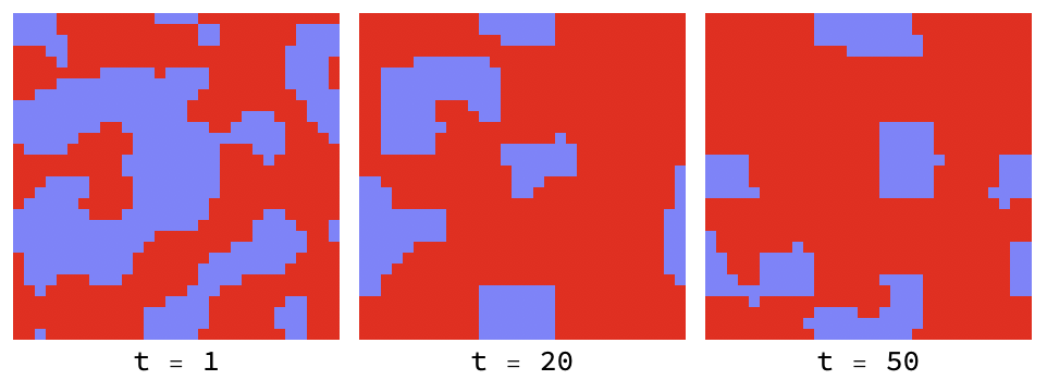
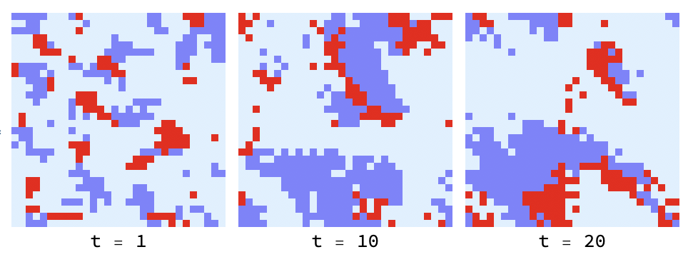
If the ’temperature’ is low enough, defectors (red) cannot penetrate virtuous clusters of co-operators (blue):

Higher temperatures allow fluctuations to help defectors (red) infiltrate and destroy clusters of co-operators (blue):

The introduction of a ’neutral’ strategy (light blue) which is the equivalent of “not playing the game” results in quite different dynamics and much more friendliness all around:

Clustering

Simulate[
	InitialPopulation -> Randomized[{0, 1, 2, 3}],
	Payoff -> Function[{x, cells}, Count[cells, x]/Length[cells]], 
	AgentType -> "Constant", Neighborhood -> 6, Temperature -> 1]

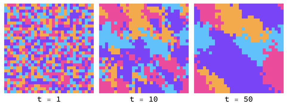
In this game, the payoff is simply how many of an agent’s neighbors are the same as it. This rewards the formation of local patches in which all agents choose the same strategy. Here is an example with 5 possible strategies that are initially randomly distributed that later coalesce into larger groups:

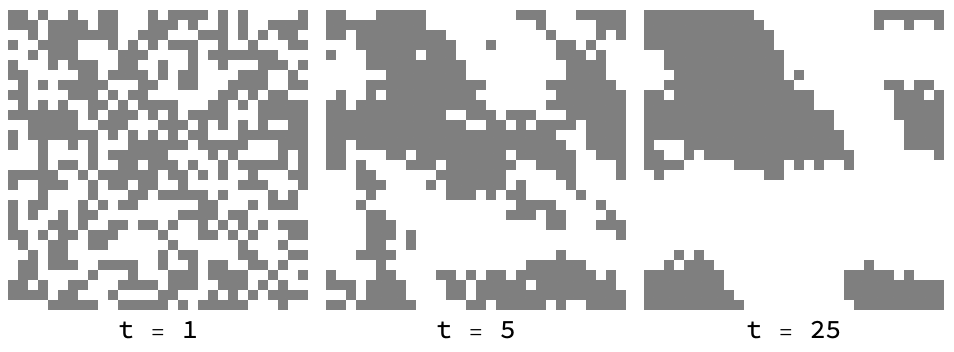
Ising model

Simulate[
	InitialPopulation -> Randomized[{0, 1}],
	Payoff -> Matrix[{{1, -1}, {-1, 1}}],
	PredictiveSelection -> {0, 1},
	Payoff -> RockPaperScissors, AgentType -> "Constant",
	Temperature -> 1/3]

In statistical physics, “toy models” are often constructed to better understand the principles underlying physical phenomena. One example of a toy model is the Ising modelWikipedia, which is used to model the process by which substances like iron can acquire magnetization. Although this system has nothing to do with game theory, we can phrase it in such terms to perform a simulation with the existing code.

In this analogy, individual agents are ‘atoms’ or domains considered to be either ‘spin up’ or ‘spin down’. In the ferromagnetic case, matching neighbors have lower energy, which encourages spins to align in groups and give rise to areas of net magnetisation, even though the system started in a symmetric (random) state. The twist in this case is that the PredictiveSelection option to Simulate is used to ensure that the agent selection is no longer local – all agents can choose any strategy (spin up or down) according to what would have given the best outcome (= lowest energy) in the previous round.

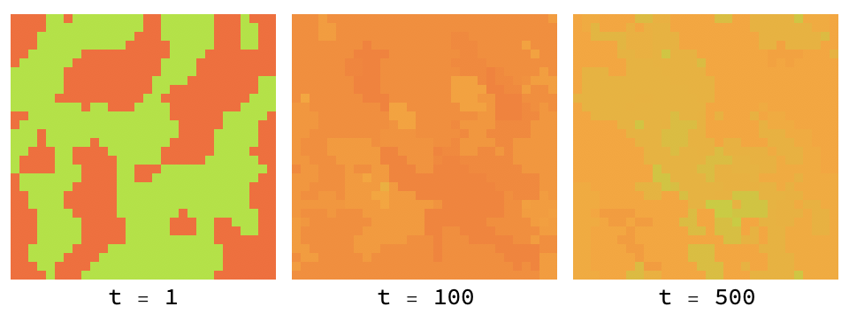
Evolution

Simulate[
	InitialPopulation -> Randomized[{_ -> Poisson[0.15], _ -> Poisson[0.85]}, "Smoothing" -> 2],
	Payoff -> Matrix[{{-2, 4}, {-4, 2}}],
	Actions -> {0, 1}, AgentType -> "Complex",
	Steps -> 1 ;; 500, Temperature -> 1/5,
	MutationRate -> 0.005]

Mutations can randomly occur when a strategy is copied from one agent to another. In this example, we have Prisoner’s Dilemma in which the players choose their actions probabilistically. Agents are shown colored according to their corresponding probability of co-operating, where bright red = always defect and bright green = always cooperate.

Interestingly, the initial group of co-operators dies out, but the remaining defectors gradually mellow until they are playing with slightly above .5 chance of co-operating (as indicated by the light orange color). Unlike one-shot Prisoner’s Dilemma (in which the only Nash equilibrium is mutual defection), the existence of gradual mutation seems to allow natural selection to slowly ‘rachet up’ the level of co-operation.

Background

About evolutionary spatial game theory

Evolutionary spatial game theory is a type of model in which ‘agents’ on a grid compete with their neighbors according to different strategies – this is the “spatial” part. Successful agents spread their strategies to their neighbors according to the degree of their relative success – this is the “evolutionary” part. The key point is that there are two things going on: there are agents playing games with each-other, and then there is the “meta-game” of natural selection acting on those agents themselves.

About the SGT package

SGT is a Mathematica package to unlock effortless explorations in evolutionary spatial game theory. Using SGT, you can setup, conduct and visualize experiments using a small number of functions and symbolic expressions to specify the initial distribution of agents, the topology of the grid, the strategies the agents employ, the payoff structure of the games they play, the rules used to update the agents and apply natural selection, whether and how mutation occurs, whether agents have access to more or less information about their opponents, and whether their success depends on global as well as local properties.

Why Mathematica?

Mathematica is a closed platform but on the other hand a very powerful tool for prototyping and building algorithms. The excellently designed core functional language, the support for graphics production and export, and finally the myriad built-in data analysis and visualization algorithms make this a very productive environment to do science in. The notebook document format is also the perfect type of interface to do exploratory work.